Simulate targets for a specific sky area (and get expected rates)#
Sometime, you do not want to simulate target for the entire sky but only for a specific part of the sky. We call that a skyarea. This skyarea is supposed to be a shapely.(Multi)Polygon and can be directly provided in the draw() (or from_draw()) method of a transient. As such, it will be passed to any fucntion that have skyarea as their parameters. This is notably the case of skysurvey.tools.random_radec() that is communly used to get the simulated target coordinates.
This is particularly useful when dealing with deep-field surveys that only observe specific fields in the sky.
Load a mock GridSurvey having 5 deep-fields#
import skysurvey
from skysurvey import examples
survey = examples.get_mock_gridsurvey()
fig = survey.show(autoscale=True)
.get_skyarea()#
GridSurveys have a get_skyarea() method that returns a (Multi)Polygon corresponding to each of its observing field. This is a shapely.geometry
skyarea = survey.get_skyarea()
skyarea

.get_timerange()#
Survey also have a .get_timerange() method that provide the fist and last observation.
tstart, tstop = survey.get_timerange()
.from_draw(skyarea=, tstart=, tstop= )#
Hence, you can simply load a transient using these three keywords
targets = skysurvey.SNeIa.from_draw(tstart=tstart, tstop=tstop,
                                    skyarea=skyarea,
                                    zmax=1)
from cartopy import crs
origin = 180
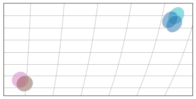
fig = survey.show(autoscale=True, origin=origin)
# Show overlapping targets, we use the crs.PlateCarree() for the non-healpy survey.show()
ax = fig.axes[0]
ax.scatter(targets.data["ra"].values-origin, targets.data["dec"].values,
transform=crs.PlateCarree(), # Important !
alpha=0.9, s=3, lw=0)
<matplotlib.collections.PathCollection at 0x2a1c1ff10>
skyarea.buffer()#
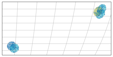
Since skyarea is a shapely.(Multi)Polygon, it has a buffer method, if you want to simulate targets around the fields.
Let’s say we want to simulate 2 degrees around the fields and not just overlapping the fields.
simply do:
targets = skysurvey.SNeIa.from_draw(tstart=tstart, tstop=tstop,
                                    skyarea=skyarea.buffer(2),
                                    zmax=1)
from cartopy import crs
origin = 180
fig = survey.show(autoscale=True, origin=origin)
# Show overlapping targets, we use the crs.PlateCarree() for the non-healpy survey.show()
ax = fig.axes[0]
ax.scatter(targets.data["ra"].values-origin, targets.data["dec"].values,
          transform=crs.PlateCarree(), # Important !
          alpha=0.9, s=3, lw=0)
<matplotlib.collections.PathCollection at 0x2a1b8c580>

No size provided, how come ?#
Transients like SNeIa have a pre-defined rate (see targets.rate), hence, given tstart and tstop, the draw() method derives nyears. Then, given the inputs skyarea and zmax, it computes size.
tip: you can combine tstop + nyears (-> tstart) | tstart + nyears (->tstop). If you provide both nyears and size, nyears will be ignored for the size computation.
tip: using skyarea and nyears, you can
targets.rate # volumetric rate, in Gyr^3/year
23500.0
Using skyarea and nyears to get a quick look at how many targets should exist#
You can combine skyarea and nyears to have a quick look at how many targets are supposed to be created by nature up to a given redshift (or redshift shell).
Say you want to know how many targets nature should create, in 3 years, for a 9deg^2 fields between \(z\in[0.3,0.6]\)
from shapely import geometry
skyarea = geometry.box(0, 0, 3, 3)
print(skyarea.area)
skyarea
9.0

snia= skysurvey.SNeIa.from_draw(nyears=3, skyarea=skyarea, zmin=0.3, zmax=0.6)
len(snia.data)
635
So: 635 SNeIa !